What is Symplectic Geometry? — Part 1

Since starting my PhD in symplectic geometry, my answer to the question to what I am doing has gotten more complicated. (Before I was mainly interested in knot theory, which offers itself to some more intuitive explanations.) So I decided to give the usual answer in this post.

Like many mathematical topics, symplectic geometry has its origin in physics, more specifically classical mechanics, that is the part of physics you may have learnt in school, where we ignore the effects of relativity and quantum mechanics. This is for example a good model to describe the movement of the planets in the solar system, or a ball flying through the air.

So what are the ingredients we need to describe what will happen to some system? Let’s take for example the pendulum: We have a weight fixed on one end of a stiff rod which is fixed at the other end, with gravity pulling down the weight. To be able to predict what happens next to the pendulum, we need to know to things: Where it currently is, and how fast it is currently going. For example if we know that the pendulum is currently at the bottom of the swing, and additionally that is has 0 speed, we know it will just hang stationary. However if we know that it is going with some speed to the right, we know it will swing up to the right, until it turns around, going through the bottom but in the other direction.

So to see everything that might be going on in our system we can look at the configuration space of our system, where each point represents a position and speed. In case of the pendulum this space is a cylinder: The position takes values on a circle, while the velocity at any point of the circle can be anything from stationary to super fast in either direction, thus some number.

The nice thing about the configuration space is that here we can see the total future development of the state. This is called the “orbit” of a point in the configuration space.

For example for green the state in the picture above, we know that the weight will fall back down to the middle while increasing its velocity, then rise back up on the other side, losing velocity until it turns back around, falling back towards the middle while now gaining velocity in the other direction. In our pendulum we are ignoring any friction or air resistance, so in this idealized situation, the weight swings back to its original state.

Now the configuration space allows us to look at all the orbits simultaneously:

Here is a fantastic website where you can see the points in the configuration space flowing along their orbits. (There the cylinder is “unwrapped” and repeated in the vertical direction.)

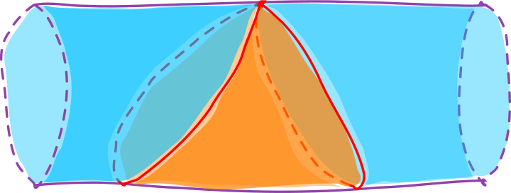
The orange region corresponds to the pendulum swinging back and forth, however once we have enough speed, the pendulum will go over the highest point and fall down on the other side again. We find these orbits in the blue region, we can imagine this global behaviour of all the points on the configuration space as some “flow”, as if it were some liquid moving along the orbit lines.

Between these two classes of orbits are two very special orbits. They are somehow an artefact of our choice to ignore air resistance or friction. It is the orbits where the pendulum has exactly the right amount of velocity to reach the top of the circle, but not go over it. Also since it is slowing down as it reaches the top, it will actually never get there, only getting closer and closer. And there is a third weird orbit, the one where the pendulum balances at the top of the swing, without falling down.

These orbits are a bit weird, because we would not be able to observe them in reality. You’re instinct may be to try to fix our model by introducing friction or air resistance, but this is not really the point of mathematics. Rather than trying to make our model more complicated by mimicking reality more closely, we will try to make our model more simple, while perhaps abandoning the desire to model reality too closely.

So in the next post we’ll try to boil down our problem to the essence: Given some configuration space (maybe or maybe not of a real physical system), exactly what is needed to translate an energy function into a “flow” of points of that configuration space?